Malvecdb: Malware and Vectorstores for semantic querying
Introduction
On Twitter, I see this article from Akamai: Patch Wednesday: Analysis with LLMs. In this article, Akamai discuss using a multi-agent system to do some stuff with CVEs - they showed this diagram.
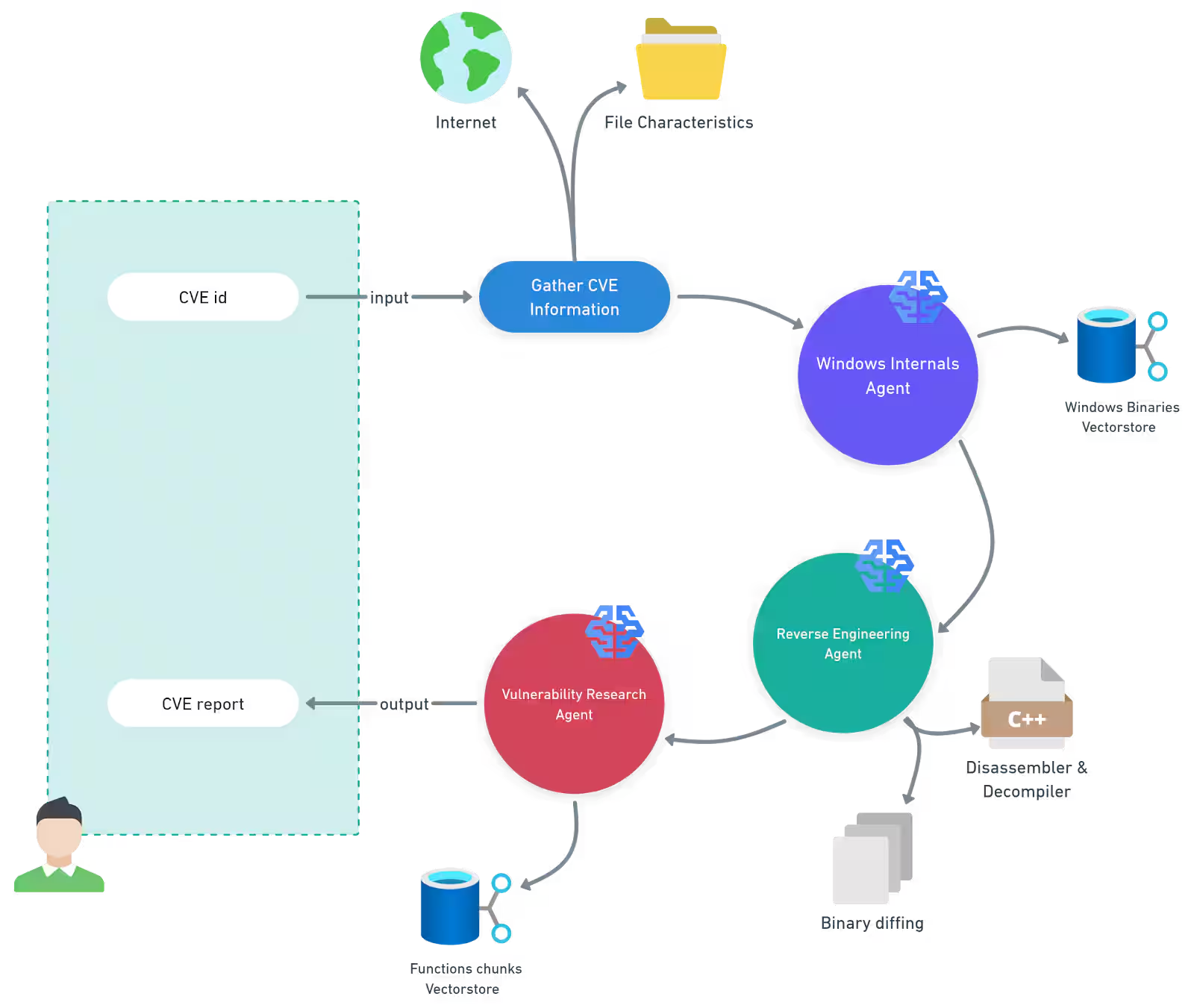
As fun as all that looks, the bit that caught my attention was the Windows Binaries Vector store - quote:
Windows internals agent — This agent uses a retrieval-augmented generation (RAG) pipeline backed by a vector store containing Windows binaries and their functionality metadata. This enables the agent to significantly narrow the scope of analysis and focus on the most relevant components.
To me, this sounded really cool and being able to query a dataset of malware and ask questions semantic questions could be interesting. Examples:
- give me every sample where GetProcAddress is imported and the binary is less than 1KB
- give me every sample that has an entropy higher than 6.5 and has a UPX section
- etc.
I had no idea you could do this with malware so I began looking it up and put something together to do this.
So, in this blog, I want to utilise the dataset I've mentioned a few times this year and build this out to run some semantic queries. Here are the blogs referencing this dataset:
- Citadel: Binary Static Analysis Framework
- Citadel 2.0: Predicting Maliciousness
- Using EMBER2024 to evaluate red team implants
- Static Data Exploration of Malware and Goodware Samples
Goal
At a high level, this boils down to a simple question:
"What is similar to this, when I don't yet know what I'm looking for?"
The context for this matters a lot and the scenario is:
- I found a weird thing
- What looks similar to this
Step 1: Structured queries
Before doing anything, the first step is to parse an PE into something structure. In this case, the PE is already structured so its just a case of taking that model and converting it into something like JSON. No vectors yet. No LLMs. Just hard constraints.
As its JSON, each sample can be shoved into Mongo DB and queried for things like:
{"entropy": { "$gt": 7.5 }}Step 2: Similarities
Let's say we query the data and from 700,000 we get a new list of 200 samples. Now we want to group them and ask how similar do they look or expand it back out to the 700,000 and potentially match things we missed. Once the data is constrained to a subset, then its a case of doing things like:
- nearest-neighbor searches
- clustering
- outlier detection
Step 3: Insight (the actual research output)
The final step, for this variant, is to visualise and filter. For that, streamlit was used - more on that later.
Putting it together
When all stitched together, a conceptual workflow would look like this:
# 1. Hard filter (Mongo)
candidates = mongo.find({
    "file_features.overall_entropy": {"$gt": 7.5},
    "imports": {
        "$all": [
            "KERNEL32.dll!GetProcAddress",
            "KERNEL32.dll!LoadLibraryA"
        ]
    }
})

candidate_ids = [c["sha256"] for c in candidates]

# 2. Similarity expansion (Chroma)
neighbors = chroma.query(
    where={"sha256": {"$in": candidate_ids}},
    n_results=20
)
Before building, some background information.
Windows Binary Vector store
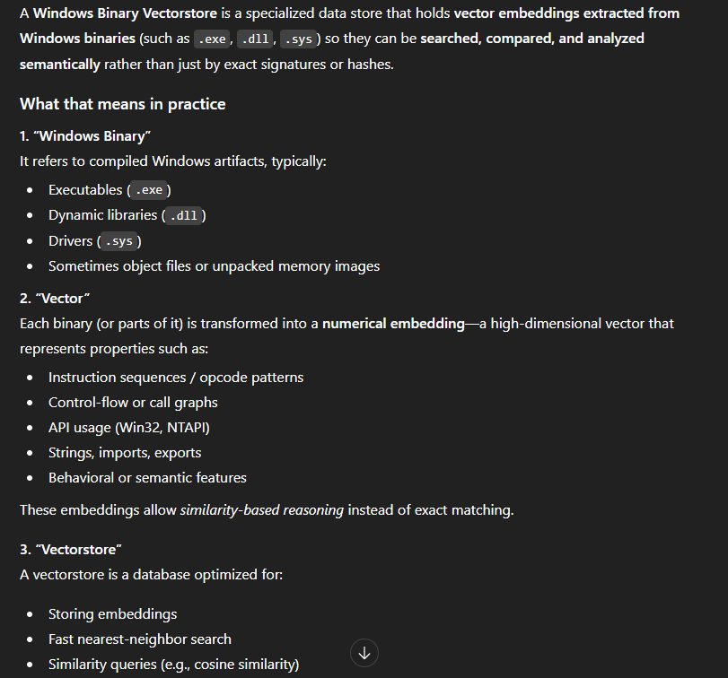
As all good research in 2025 starts, I asked the AI to explain what a Binary Vector store was.
The response from this was as expected, some ramblings on vector embeddings which is something I've written about before in From RAGs to Riches: Using LLMs and RAGs to Enhance Your Ops, and we can see a pretty good definition for vector store's in this MongoDB article: Vector Stores in Artificial Intelligence (AI)
MongoDB explain it best:
Typically found in vector databases, a vector store is a digital storage system that holds vectors – the unique fingerprint for a piece of data, whether it's a sentence, an image, or a user's browsing habits. The vector store not only keeps these vectors together in a vector space, but also quickly and efficiently finds and places similar vectors or identical vectors near one another.
...
In artificial intelligence, a vector is a mathematical point that represents data in a format that AI algorithms can understand. Vectors are arrays (or lists) of numbers, with each number representing a specific feature or attribute of the data. They are housed in vector stores and used in vector databases in AI applications.
In simple terms, vectors are numerical representations of data.
Vectors and Distances
Before we get anywhere near malware, CVEs, or Windows binaries, it's worth grounding this in the most basic possible example. A vector is just a list of numbers. Each number represents something about the thing you're describing, and as long as you're consistent, you can start doing useful maths over the top of it. In the example below, I've made up three attributes for animals, size, speed, and lifespan from the MongoDB blog, and represented each animal as a 3-dimensional vector. A mouse becomes [1, 8, 2], an elephant becomes [10, 3, 60]. The values themselves don't matter too much; what matters is that similar things look similar numerically.
| Animal | Size | Speed | Lifespan |
|---|---|---|---|
| Mouse | 1 | 8 | 2 |
| Cheetah | 5 | 10 | 12 |
| Rabbit | 2 | 9 | 8 |
| Elephant | 10 | 3 | 60 |
| Turtle | 3 | 1 | 80 |
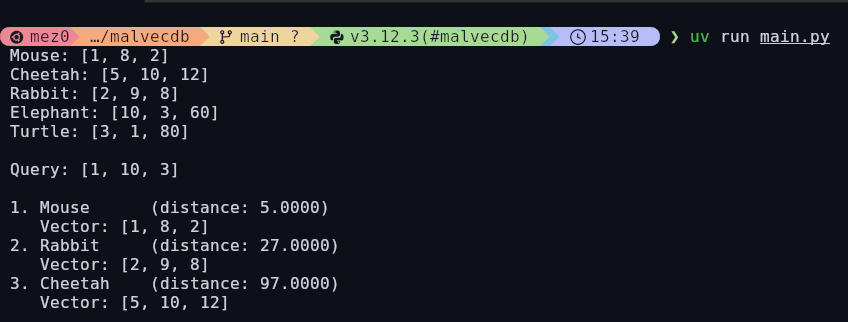
Once you've got data in this format, you can stop asking "does this match?" and start asking "what's closest?". The query vector [1, 10, 3] roughly describes something small, very fast, and short-lived. When we ask the vector store to find the nearest neighbours, it calculates the distance between that query and every stored vector and sorts them. Unsurprisingly, the mouse comes out on top, followed by the rabbit and then the cheetah.
Here is the code for that:
import chromadb

client = chromadb.Client()
animals = client.create_collection("animals")

animal_data = {
    "Mouse": [1, 8, 2],  # small, fast, short-lived
    "Cheetah": [5, 10, 12],  # medium, very fast, medium-lived
    "Rabbit": [2, 9, 8],  # small, fast, medium-lived
    "Elephant": [10, 3, 60],  # large, slow, long-lived
    "Turtle": [3, 1, 80],  # medium, very slow, very long-lived
}

for name, embedding in animal_data.items():
    print(f" {name}: {embedding}")

animals.add(
    ids=list(animal_data.keys()),
    embeddings=list(animal_data.values()),
)

query_vector = [1, 10, 3]  # small, very fast, short-lived

print()

print(f" Query: {query_vector}")

results = animals.query(query_embeddings=[query_vector], n_results=3)

print()

for i, (animal_id, distance) in enumerate(
    zip(results["ids"][0], results["distances"][0]), 1
):
    embedding = animal_data[animal_id]
    print(f" {i}. {animal_id:10} (distance: {distance:.4f})")
    print(f"    Vector: {embedding}")
Here is the full results:
{
    "ids": [
        [
            "Mouse",
            "Rabbit",
            "Cheetah"
        ]
    ],
    "embeddings": null,
    "documents": [
        [
            null,
            null,
            null
        ]
    ],
    "uris": null,
    "included": [
        "metadatas",
        "documents",
        "distances"
    ],
    "data": null,
    "metadatas": [
        [
            null,
            null,
            null
        ]
    ],
    "distances": [
        [
            5.0,
            27.0,
            97.0
        ]
    ]
}
In the image above, we can see mouse has a distance of 5, rabbit is 27, and cheetah is 97. By default, ChromaDB default's to L2 Squared Distance which is detailed under the collection properties:
Blogs such as ChromaDB Defaults to L2 Distance — Why that might not be the best choice state that changing to "cosine" have a 10x improvement. This section is a little out of scope for what I want to do, so I would suggest reading the blog linked above, and check out this one from Elastic: Understanding the approximate nearest neighbor (ANN) algorithm. It may also be worth reading papers like A Comprehensive Survey on Vector Database: Storage and Retrieval Technique, Challenge.- distance metric - by default Chroma use L2 (Euclidean Distance Squared) distance metric for newly created collection. You can change it at creation time using `hnsw:space` metadata key. Possible values are `l2`, `cosine`, and 'ip' (inner product). (Note: `cosine` value returns `cosine distance` rather then `cosine similarity`. Ie. values close to 0 means the embeddings are more similar.)
Note: I am not getting into the weeds of Vector vs. KNN. Mainly because I am not entirely sure.
Vectored Malware
Every time I look up some papers for malware, Robert J. Joyce appears. When researching for this blog, I was looking for "vector datastore" + "malware" and found: AVScan2Vec: Feature Learning on Antivirus Scan Data for Production-Scale Malware Corpora. In this paper, the researchers use a vectored approach to map anti-virus data for ease-of-searching, very similar to what I want to do. This graphic from the paper illustrates the process.
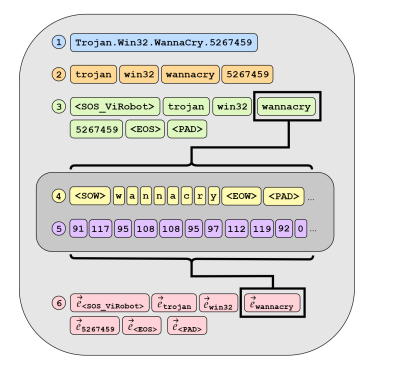
What I found cool in this paper is the ability to do behavioural tag classification:
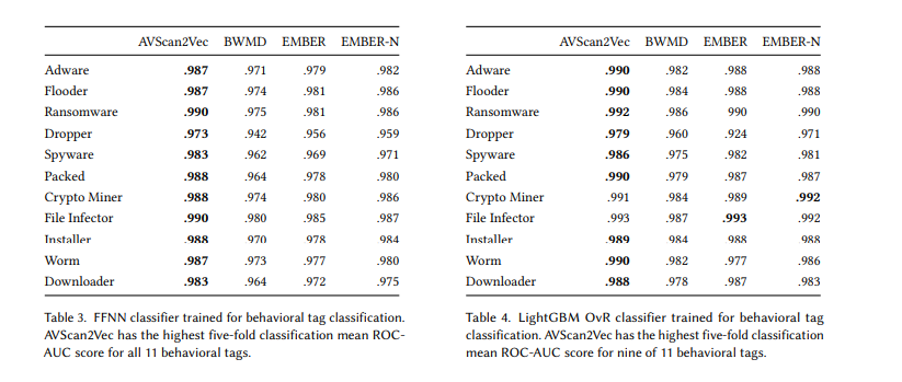
At scale, its pretty fun to have a sample and then get an approximate malware-tag bag. For example:
- Upload Sample
- .990 that this is ransomware
AVScan2Vec was useful for me not because I want to replicate it, but because it validated the core idea of representing malware as vectors and then reasoning about similarity at scale actually works. That paper operates at the antivirus telemetry layer, embedding how engines describe a sample rather than what the binary itself contains. My interest sits one layer lower. Instead of learning from AV opinions, I want to embed properties extracted directly from Windows binaries such as imports, sections, entropy, sizes, strings, and other static features, and then throw those into a vector store I can query myself.
Dataset, PE Parsing, and Chroma
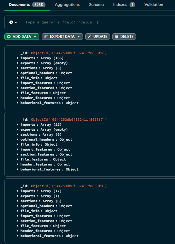
The dataset here is largely from Static Data Exploration of Malware and Goodware Samples and it is already processed - here is an example.
For the most part, the PE parsing has been discussed in the original citadel blog. However, this will all be done with lief.
Here is an example of a parsed PE:
{"imports": ["MSVCRT.dll!memset", "SHLWAPI.DLL!PathGetArgsA", "..."], "exports": [], "sections": [{"name": ".code", "size": 13824, "entropy": 5.280707524399077}, {"name": ".text", "size": 47616, "entropy": 6.59538319470133}, {"name": ".rdata", "size": 2560, "entropy": 6.7945349341395085}, {"name": ".data", "size": 5632, "entropy": 5.514372950569856}, {"name": ".rsrc", "size": 68096, "entropy": 7.978753539651748}], "optional_headers": {"addressofentrypoint": 4096, "baseofcode": 4096, "baseofdata": 69632, "checksum": 0, "filealignment": 512, "imagebase": 4194304, "loaderflags": 0, "magic": "PE32", "majorimageversion": 0, "majorlinkerversion": 2, "majoroperatingsystemversion": 4, "majorsubsystemversion": 4, "minorimageversion": 0, "minorlinkerversion": 50, "minoroperatingsystemversion": 0, "minorsubsystemversion": 0, "numberofrvaandsize": 16, "sectionalignment": 4096, "sizeofcode": 61440, "sizeofheaders": 1024, "sizeofheapcommit": 4096, "sizeofheapreserve": 1048576, "sizeofimage": 151552, "sizeofinitializeddata": 76288, "sizeofstackcommit": 4096, "sizeofstackreserve": 1048576, "sizeofuninitializeddata": 0, "subsystem": "WINDOWS_CUI", "win32versionvalue": 0}, "file_info": {"sha256": "0000015bf5f766e7a709983fe08a8d6983fb5d49213d4389871c2b69e6c19b25", "size": 138752, "entropy": 7.486094089884453}, "import_features": {"has_imports": true, "total_import_count": 166, "kernel32_count": 58, "ntdll_count": 0, "advapi32_count": 0, "user32_count": 61, "ws2_32_count": 0, "winhttp_count": 0, "wininet_count": 0, "category_counts": {"process_thread_mgmt": 38, "network_ops": 1, "memory_mgmt": 12, "registry_ops": 0, "file_ops": 21, "crypto_ops": 1, "dll_injection": 7, "hooking_interception": 4, "system_info_control": 34, "graphics_ops": 0, "security_ops": 0}, "category_ratios": {"process_thread_mgmt_ratio": 0.2289156626506024, "network_ops_ratio": 0.006024096385542169, "memory_mgmt_ratio": 0.07228915662650602, "registry_ops_ratio": 0.0, "file_ops_ratio": 0.12650602409638553, "crypto_ops_ratio": 0.006024096385542169, "dll_injection_ratio": 0.04216867469879518, "hooking_interception_ratio": 0.024096385542168676, "system_info_control_ratio": 0.20481927710843373, "graphics_ops_ratio": 0.0, "security_ops_ratio": 0.0}, "has_injection_apis": true, "has_registry_apis": false, "has_network_apis": true, "has_crypto_apis": true, "has_hooking_apis": true, "import_entropy": 2.1205749752446783, "injection_without_network": false, "crypto_with_network": true}, "section_features": {"section_count": 5, "total_section_size": 137728, "has_text": true, "has_data": true, "has_rdata": true, "has_rsrc": true, "has_reloc": false, "has_upx": false, "has_aspack": false, "has_themida": false, "has_vmprotect": false, "min_entropy": 5.280707524399077, "max_entropy": 7.978753539651748, "avg_entropy": 6.432750428692304, "entropy_variance": 0.9436166219425252, "high_entropy_section_count": 1, "min_size": 2560, "max_size": 68096, "avg_size": 27545.6, "text_size_ratio": 0.34572490706319703, "has_zero_size_sections": false, "has_executable_rsrc": true, "has_unusual_names": true, "section_count_anomaly": false}, "file_features": {"size_bytes": 138752, "is_tiny": false, "is_small": false, "is_medium": true, "is_large": false, "is_huge": false, "overall_entropy": 7.486094089884453, "is_low_entropy": false, "is_moderate_entropy": false, "is_high_entropy": false, "is_packed_entropy": true, "size_normalized": 0.013232421875, "entropy_normalized": 0.9357617612355567}, "header_features": {"is_64bit": false, "is_dll": false, "is_console": true, "is_gui": false, "is_stripped": true, "has_code_signature": false, "timestamp_year": 0, "is_recent_compile": false, "entrypoint_offset_ratio": 0.02702702702702703, "code_to_data_ratio": 0.44609665427509293, "imagebase_is_default": true, "addressofentrypoint": 4096, "sizeofcode": 61440, "sizeofinitializeddata": 76288, "sizeofimage": 151552, "sectionalignment": 4096, "filealignment": 512, "majorlinkerversion": 2, "minorimageversion": 0, "checksum": 0, "sizeofheaders": 1024, "numberofrvaandsize": 0}, "behavioral_features": {"injection_score": 0.0, "stealth_score": 1.0, "persistence_score": 0.0, "data_theft_score": 1.0, "is_signed": false, "has_overlay": false, "has_resources": true, "has_debug_info": false, "packer_confidence": 1.0, "risk_score": 0.5}}At a high level, this pipeline is about projecting structured PE features into a semantic space that can be searched and compared meaningfully. After parsing each binary into rich, structured JSON (imports, entropy, sections, behavioural indicators, headers, etc.), the code converts that data into a deterministic natural-language description and then embeds that description using a sentence-level transformer model.
The embedding step relies on the sentence-transformers library:
from sentence_transformers import SentenceTransformer

self.model = SentenceTransformer("all-MiniLM-L6-v2")
By default, the pipeline uses all-MiniLM-L6-v2, a compact transformer model that produces 384-dimensional embeddings trained via contrastive learning. The model is not malware-specific; instead, it is optimized to place semantically similar sentences close together in vector space. That's a deliberate design choice: rather than training a bespoke model, we translate malware features into language and let a well-trained semantic model handle the alignment. Using the example code:
from sentence_transformers import SentenceTransformer
sentences = ["This is an example sentence", "Each sentence is converted"]

model = SentenceTransformer('sentence-transformers/all-MiniLM-L6-v2')
embeddings = model.encode(sentences)
print(embeddings)
embeddings here is (snipped):
[[ 6.76569268e-02  6.34959638e-02  4.87131029e-02  7.93049783e-02
   3.74480858e-02  2.65278737e-03  3.93749885e-02, ...]]
The key design pattern here is a mad-lib–style text generator. Every sample is mapped into the same narrative skeleton:
This binary imports {APIs}.
It shows {capabilities} with a risk score of {x}.
The binary is {packed/unpacked}.
File entropy is {y} and size is {z}.
{architecture, file type, and subsystem}.
What you end up with is not a replacement for classical feature vectors or rule-based querying, but a semantic overlay. Precise predicates like "entropy > 7.5 AND imports LoadLibraryA" still belong in a structured store such as MongoDB. The embedding layer answers a different question: "what other binaries look like this one?" or "show me samples with similar operational intent." By keeping the text generation deterministic and the model fixed, this approach yields reproducible, explainable similarity search on top of traditional malware analysis primitives—bridging exact filtering and fuzzy, intent-level reasoning in a single workflow.
Overall, this produced 698,045 parsed PE files which were then loaded into Chroma DB with hnsw:space.

Recap
At this stage, the dataset has been parsed into structured PE metadata and stored in MongoDB as the system of record. This allows for explainable filtering using traditional queries like overall_entropy > 7.5 or imports contains LoadLibraryA).
Each sample is deterministically translated into a natural-language description and embedded using all-MiniLM-L6-v2. These embeddings are stored in ChromaDB and act as a semantic index over the dataset.
This gives us two capabilities:
- MongoDB for exact, logic-based selection of samples.
- ChromaDB for similarity search across the selected samples, answering questions like "what other binaries behave like this one?"
This mirrors the approach described in Akamai's bin diff work from the start of this blog: structured analysis provides the facts, while embeddings provide a way to reason about similarity and intent at scale.
MongoDB Queries
The first step once the JSON documents are loaded into Mongo DB is to bring the number of samples down from 698,000 to anything more approachable.
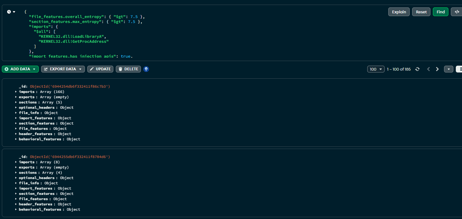
To do that, I crafted a naive query to find any samples with high entropy, and then two imported functions: LoadLibraryA and GetProcAddress. This is essentially being lazy and looking for things that might potentially be doing some runtime function resolution with a payload inside it.
{
"file_features.overall_entropy": { "$gt": 7.5 },
"section_features.max_entropy": { "$gt": 7.5 },
"imports": {
"$all": [
"KERNEL32.dll!LoadLibraryA",
"KERNEL32.dll!GetProcAddress"
]
},
"import_features.has_injection_apis": true,
"header_features.is_console": true,
"header_features.is_dll": false
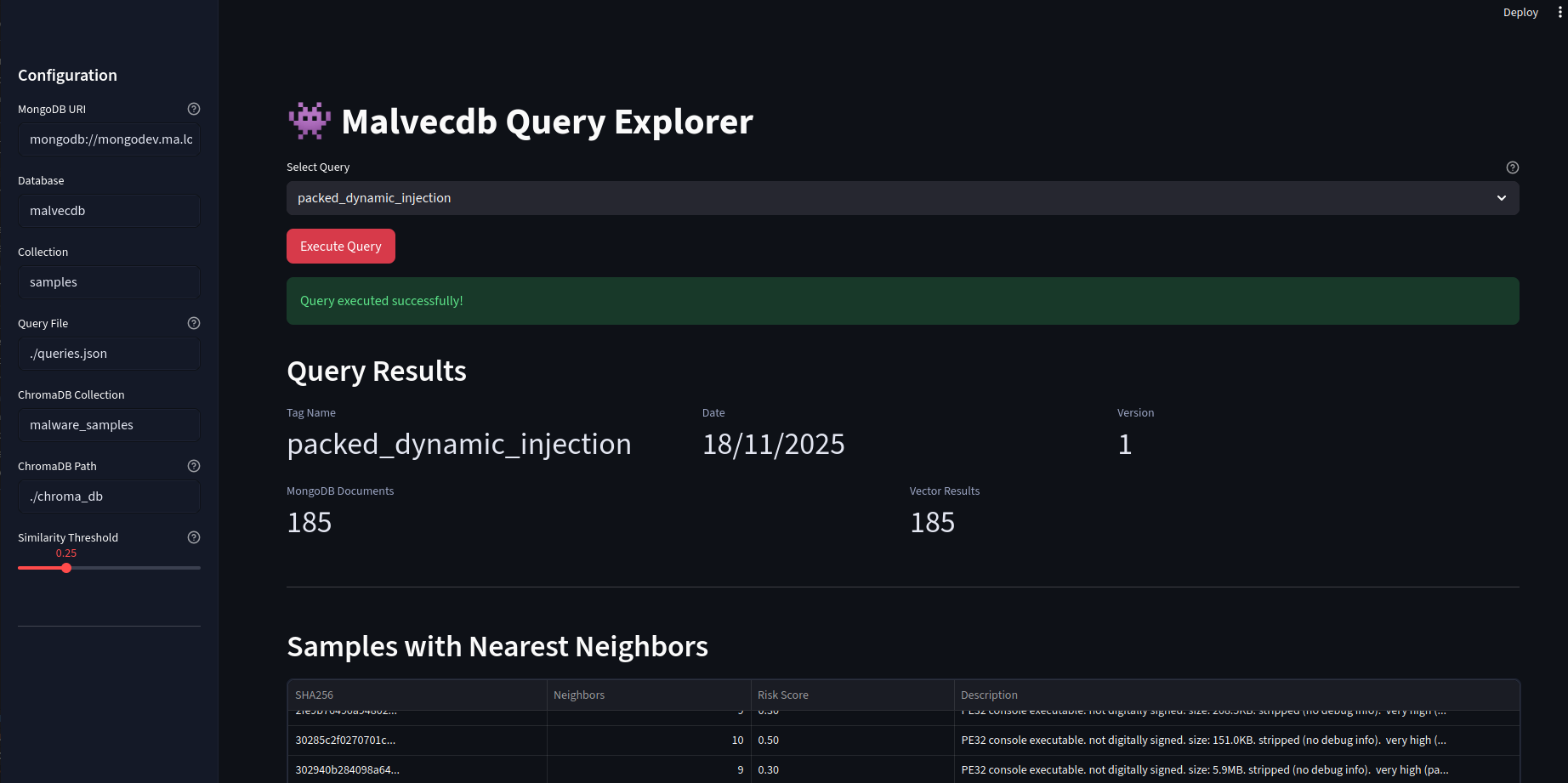
}Firing this off returns 185 results. This is good, its proving to be a valid logic gate.
At this point, I had an idea to then create a structure which mapped the query to a "tag" with extra metadata. I aptly named this one packed_dynamic_injection - not quite accurate, but its a POC.
{
  "packed_dynamic_injection": {
    "date": "18/11/2025",
    "version": 1,
    "query": {
      "file_features.overall_entropy": {
        "$gt": 7.5
      },
      "section_features.max_entropy": {
        "$gt": 7.5
      },
      "imports": {
        "$all": [
          "KERNEL32.dll!LoadLibraryA",
          "KERNEL32.dll!GetProcAddress"
        ]
      },
      "import_features.has_injection_apis": true,
      "header_features.is_console": true,
      "header_features.is_dll": false
    }
  }
}
With that, the next thing is to create the embedding. Consider this:
import random

descriptions = ["stinky", "smelly", "fat", "thin"]

nouns = [
    "dog",
    "cat",
    "bird",
    "fish",
    "horse",
    "rabbit",
    "snake",
    "tiger",
    "lion",
    "bear",
]

verbs = [
    "runs",
    "walks",
    "flies",
    "swims",
    "jumps",
    "runs",
    "walks",
    "flies",
    "swims",
    "jumps",
]

adverbs = [
    "quickly",
    "slowly",
    "angrily",
    "happily",
    "sadly",
    "excitedly",
    "calmly",
]

directions = [
    "towards the",
    "from the",
    "in the",
    "out of the",
    "around the",
    "behind the",
    "in front of the",
    "under the",
    "above the",
]

locations = [
    "park",
    "school",
    "library",
    "hospital",
    "mall",
    "restaurant",
    "bar",
]

madlib = "The {description} {noun} {verb} {adverb} {direction} the {description} {noun}s in the {location}."

print(
    madlib.format(
        description=random.choice(descriptions),
        noun=random.choice(nouns),
        verb=random.choice(verbs),
        adverb=random.choice(adverbs),
        direction=random.choice(directions),
        location=random.choice(locations),
    )
)
Then:
The smelly snake runs calmly around the the smelly snakes in the restaurant.The next step is this, but for malware:
PE32 console executable. SHA256: 00c09a5e167016acc669f694f82962639d619f449d0705749dbe6ed156d8adb8. linker version 2.50. targets OS version 4.0. subsystem version 4.0. not digitally signed. invalid or missing checksum. size: 150.0KB. stripped (no debug info). very high (packed/obfuscated) overall entropy (7.55) 1 high-entropy section(s) average section entropy: 6.43 (variance: 0.94) likely packed or obfuscated (high entropy without known packer signature) 5 section(s), unusual section names, executable .rsrc section (suspicious) sections: .code (13.5KB, entropy: 5.28), .text (46.5KB, entropy: 6.60), .rdata (2.5KB, entropy: 6.79), .data (5.5KB, entropy: 5.51), .rsrc (81.0KB, entropy: 7.97). imports 166 API(s) primarily from kernel32.dll (58), user32.dll (61) also uses: comctl32.dll, gdi32.dll, msvcrt.dll, ole32.dll, shell32.dll significant capabilities: process/thread management (38 APIs, 22.9%), memory management (12 APIs, 7.2%), file operations (21 APIs, 12.7%), system information/control (34 APIs, 20.5%) diverse DLL usage (high import entropy) capabilities: process injection with network capabilities, network-capable, cryptographic APIs with network (potential C2 encryption), API hooking/interception, extensive file operations. exhibits: stealth/evasion capabilities (score: 1.00), data theft/exfiltration capabilities (score: 1.00) threat patterns: crypto with network (suggests encrypted C2 communication), executable resources section (uncommon, potentially suspicious), unsigned high-entropy binary (common malware pattern) contains embedded resources. overall behavioral risk: high (score: 0.50) primary risk factors: stealth, data theft.Once that is loaded up into Chroma - we can move onto the visualisation step.
Visualisation
streamlit describes itself as:
faster way to build and share data apps
I heard about it long ago and never used it, so I figured this was the behalf chance for it. It basically allows for the quick creation of a web app using python. For example, it can automatically convert a dataframe to a filterable table in the UI.
The workflow up to this point has just been a python class:
uv run malvecdb.py -qf queries.json query -q packed_dynamic_injectionThis will then run the Mongo query, generate the madlib's, and return the similarities. The next step was to take this class and pipe it into Streamlit so I visually see the similarities with networkx. Let's walk through the app.
Note: I didn't write a single line of code for this. Cursor did it with one prompt
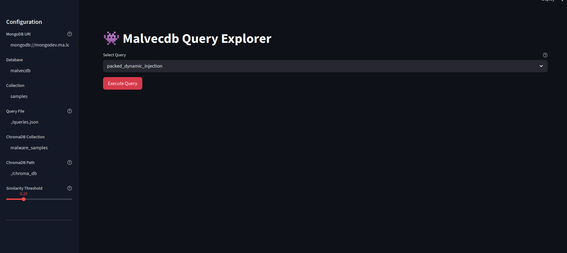
The landing page allows for the queries to the picked with a configurable sidenav. Once "Execute Query" is hit, this will fire off the Mongo query.
When it returns, we get the results and metadata in a nice table.
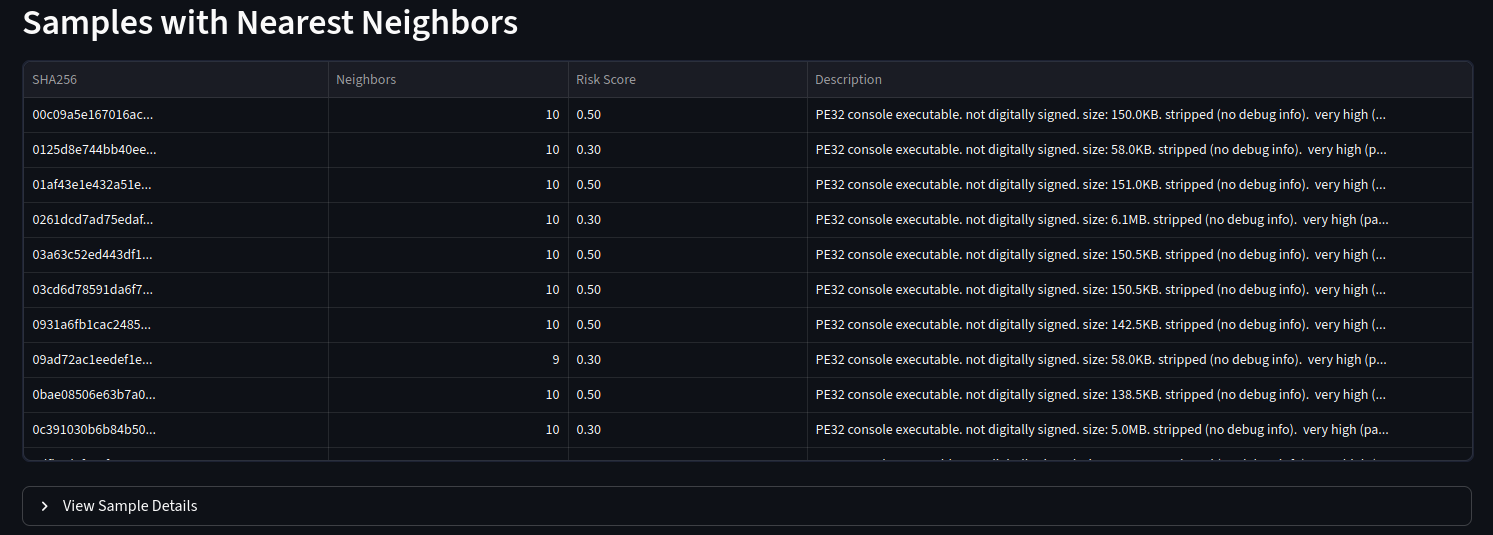
But the main event is the breathing networkx diagram. This allows for the groups to emerge which is fascinating. Clicking on a particular node will copy the hash so it can go and be looked up.
Overall, this completes my initial goal. I have some future ideas where each cluster can be subject to more interrogation, but thats not in the scope of this blog. I also plan to release the code, but I want to do some more work on it and potentially do a follow up blog.
Conclusion
This started as curiosity about a single line in an Akamai blog and ended with something that feels genuinely useful: a way to move fluidly between exact facts and approximate intent when working with large malware corpora. MongoDB gives me a place to be precise whilst the vector layer lets me ask a very different class of question: what else behaves like this?
What surprised me most is how little "AI magic" was actually required. There's no malware-specific LLM, no fine-tuning, and no opaque scoring model. The heavy lifting comes from simple structured data and modern tooling. The final product isn't a solution to anything, but it's a fun way to do some more research.